9.4 - Math for Perspective Projections¶

This lesson describes the mathematics behind a 4-by-4 perspective transformation matrix.

But first, let’s list the tasks the graphics pipeline does automatically after the projection matrix has transformed a scene’s vertices. After a vertex shader has processed a vertex, the vertex passes through the following graphic pipeline stages in the order listed:

Clipping - geometric primitives are clipped against the viewing volume. Since the “perspective division* has not been performed yet, clipping is performed on an (x,y,z) vertex that is outside the limits of -w <= x <= w, -w <= y <= w, and -w <= z <= w. Note that every vertex has a unique w value (i.e., -z).
Perspective divide - “clipping space” vertices, (x,y,z,w), are transformed into normalized device coordinates, (x/w, y/w, z/w).
Viewport transform - normalized device coordinates are converted into pixel locations in the output image.
Rasterization - determines which pixels in the output image are covered by a geometric primitive.
The active fragment shader is executed on each pixel.

What is important for our discussion of a perspective projection is that clipping is performed before “perspective division” is performed.

The Perspective Projection Matrix¶

A perspective projection transformation matrix must transform the vertices of a scene that are within a frustum into the clipping volume, which is a 2 unit wide cube shown in the image to the right. Doing this for a perspective projection is more challenging than an orthographic projection. We need to perform the following steps:

Translate the apex of the frustum to the origin.
Setup the vertices for the “perspective calculation.”
Normalize the depth values, z, into the range (-1,+1).
Scale the 2D, (x,y), vertex values in the viewing window (i.e., the near clipping plane) to a 2-by-2 unit square: (-1,-1) to (+1,+1).

Let’s discuss these tasks one at a time:

Translate the Frustum Apex to the Origin¶

A perspective frustum can be offset from the global origin along the X or Y axes. We need to place the apex of the frustum at the global origin for the perspective calculations to be as simple as possible. The apex is located in the center of the viewing window in the XY plane. Therefore we calculate the center point of the viewing window and translate it to the origin. The z value is always zero, so there is no translation for z.

mid_x = (left + right) * 0.5;
mid_y = (bottom + top) * 0.5;

1
0
0
0
0
1
0
0
0
0
1
0
-mid_x
-mid_y
0
1
*x
y
z
1
=x'
y'
z'
w'
Eq1

1
0
0
0
0
1
0
0
0
0
1
0
-(left+right)/2
-(bottom+top)/2
0
1
*x
y
z
1
=x'
y'
z'
w'
Eq2

Setup for the “Perspective Calculations”¶

We need to project every vertex in our scene to its correct location in the 2D viewing window. The 2D viewing window is the near plane of the frustum. Study the following diagram.

Perspective Calculations Project a Vertex to the Viewing Window

Notice that the vertex (x,y,z) is projected to the viewing window by casting a ray from the vertex to the camera (shown as an orange ray). The rendering location for the vertex is (x',y',near). From the diagram you can see that the y and y' values are related by proportional right-triangles. These two triangles must have the same ratio of side lengths. Therefore, y'/near must be equal to y/z. Solving for y' gives (y/z)*near (or (y*near)/z). Note that near is a constant for a particular scene, while y and z are different for each vertex in a scene. Using the same logic, x' = (x*near)/z.

To summarize, we can calculate the location of a 3D vertex in a 2D viewing window with a multiplication and a division like this:

x' = (x*near)/z
y' = (y*near)/z

To be precise, since all of the z values for vertices in front of the camera are negative, and the value of z is being treated as a distance, we need to negate the value of z.

x' = (x*near)/(-z)
y' = (y*near)/(-z)

But we have a problem. A 4-by-4 transformation matrix calculates a linear combination of terms, where each term contains a single vertex component. That is, we can do calculations like a*x + b*y + c*z + d, but not calculations like a*x/z + b*y/z + c*z*x + d. But we have a solution using homogeneous coordinates. Remember that a vertex defined as (x,y,z,w) defines a value in 4D space at the 3D location (x/w, y/w, z/w). Normally the w component is equal to 1 and (x,y,z,1) is (x,y,z). But to implement perspective division we can set the w value to our divisor, -z. This breaks the above calculations into two parts. A matrix transform will perform the multiplication in the numerator, while a post-processing step, after the matrix multiplication, will perform the division.

To perform the multiplication in the perspective calculation, we use this matrix transformation:

near
0
0
0
0
near
0
0
0
0
1
0
0
0
0
1
*x
y
z
w
=x'
y'
z'
w'
Eq3

To get the divisor, -z, into the w value, we use this transform:

1
0
0
0
0
1
0
0
0
0
1
-1
0
0
0
0
*x
y
z
w
=x'
y'
z'
w'
Eq4 - (click the multiplication sign or the equal sign to verify)

Using these two matrix transforms we can prepare the data for a “perspective divide” operation that will be performed later in the graphics pipeline.

Mapping Depth Values, `z`, to `(-1,+1)`¶

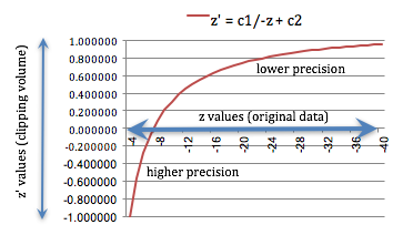
The z values in the frustum, which range from -near to -far, must be mapped to the clipping volume in a range (-1,+1). We know from our previous discussion that the homogeneous component, w, is going to be -z. We need a mapping equation that contains a division by -z. A non-linear mapping function, z' = (c1*z + c2) / -z does what we need, with a side benefit that more numerical precision is given to distances closer to the camera. [1] The required constants c1 and c2 are based on the specific range (-near,-far).

Calculating the constants `c1` and `c2`:¶

When z = -near, the mapping equation must evaluate to -1. When z = -far, the mapping equation must evaluate to +1. This gives us two equations to solve for c1 and c2.

-1 = (c1*(-near) + c2) / -(-near)
+1 = (c1*(-far) + c2) / -(-far)

Using a little algebra, we get

c1 = (far + near) / (near - far)
c2 = 2*far*near / (near - far)

Putting the `z` mapping equation into a 4x4 transformation matrix:¶

To put z' = (c1*z + c2) / -z into a 4x4 transformation matrix, the numerator goes into the matrix, while the denominator goes into the homogeneous coordinate w, like this:

1
0
0
0
0
1
0
0
0
0
c1
-1
0
0
c2
0
*x
y
z
1
=x'
y'
z'
w'
Eq5 - (click the multiplication sign or the equal sign to verify)

Non-linear mapping of z values

Note that w must be equal to 1.0 when this transform happens to get the correct mapping equation.

Let’s consider an example of the z mapping. Suppose near = 4.0 and far = 40. To the right is a plot of z values and their corresponding mapping to the range (-1,+1). Notice that the z values between -4 and -7.4 use up to half of the clipping volume values (-1.0, 0.0)! That is definitely non-linear!

Scale to the Viewing Window: `(-1,-1)` to `(+1,+1)`¶

Subsequent stages in the graphics pipeline require that the 2D viewing window be normalized to values between (-1,-1) to (+1,+1). This is easily done with a scale factor based on a simple ratio: 2/currentSize. The equations and the resulting matrix transformation are:

scale_x = 2.0 / (right - left);
scale_y = 2.0 / (top - bottom);

2/(right-left)
0
0
0
0
2/(top-bottom)
0
0
0
0
1
0
0
0
0
1
*x
y
z
w
=x'
y'
z'
w'
Eq6

Building the Prospective Projection Transform¶

Let’s put all of the above concepts together into a single perspective transformation matrix. The order of the transforms matters and we only want to put -z into the homogeneous coordinate, w, once.

Translate the apex of the frustum to the origin. (Yellow matrix)
Setup the “perspective calculation.” (Light gray matrix)
Scale the depth values, z, into a normalized range (-1,+1) and put -z into the homogeneous coordinate, w. (Purple matrix)
Scale the 2D values, (x',y'), in the viewing window to a 2-by-2 unit square: (-1,-1) to (+1,+1). (Cyan matrix)

2/(right-left)
0
0
0
0
2/(top-bottom)
0
0
0
0
1
0
0
0
0
1
*1
0
0
0
0
1
0
0
0
0
c1
-1
0
0
c2
0
*near
0
0
0
0
near
0
0
0
0
1
0
0
0
0
1
*1
0
0
0
0
1
0
0
0
0
1
0
-(left+right)/2
-(bottom+top)/2
0
1
*x
y
z
1
=x'
y'
z'
w'
Eq7

If you click on the multiplication signs in the above equation from right-to-left you can see the progression of changes to a (x,y,z,w) vertex at each step of the transformation.

If you simplify the matrix terms and make the following substitutions:

width = (right - left)
height = (top - bottom)
depth = (far - near)
c1 = -(far + near) / depth
c2 = -2*far*near / depth

the perspective transformation matrix becomes:

2*near/width
0
0
0
0
2*near/height
0
0
0
0
-(far+near)/depth
-1
-near*(right+left)/width
-near*(top+bottom)/height
-2*far*near/depth
0
Eq8

Summary¶

You will probably never implement code to create a perspective projection. The functions createFrustum() and createPerspective() in GlMatrix4x4.js implement the calculations described in this lesson. So why is this lesson’s discussion important?

There is great value in understanding the fundamentals. This lesson explained that a perspective projection is not “magical,” but rather simply a concatenation of basic transformations.
You hopefully have a better understanding of homogeneous coordinates.
The better you are at understanding, creating, and manipulating 4x4 transformation matrices, the more tools you will have at your disposal to create new and creative computer graphics.
If you want to understand complex transformations, it is very helpful if you can break them down into their elementary parts.

Glossary¶

viewing window: A rectangular 2D region on which a 3D world is projected.
perspective projection: Project all vertices of a scene along vectors to the camera’s location. Where the vector hits the 2D viewing window becomes it’s rendered location.
mapping: A function that converts a set of inputs into an output value.
linear mapping: A mapping that converts a location in one range of values to a different range while maintaining the same relative relationship between the locations.
non-linear mapping: A mapping that converts a location in one range to a different range where the location of points in the new range do not have the same relative relationship between them.

[1]	In the early days of computer graphics memory was expensive and used sparingly. The precision of values was sometimes limited to a few decimal places. Today the precision of the values is typically not an issue.

Next Section - 9.5 - Viewports